BLUEDOT Technical AI Safety Puzzle #1

Introduction

Recently BlueDot Impact put out a Technical AI Safety Puzzle [1]. The goal of this task was the understanding of a simple model, and we weren’t allowed to talk about working on the task until the puzzle closed. As an overview reminder of the structure: the BlueDot team trained a simple MLP head on top of the sentence-transformers/all-MiniLM-L6-v2 sentence embedding model, and trained it to predict whether input sentences had any of 8 classes present. The 8 classes were: number, question, color, food, sentiment, country, person and body_part. The network was trained such that the post-ReLU activations of the 3rd MLP layer were linearly separable for all but one of the classes.

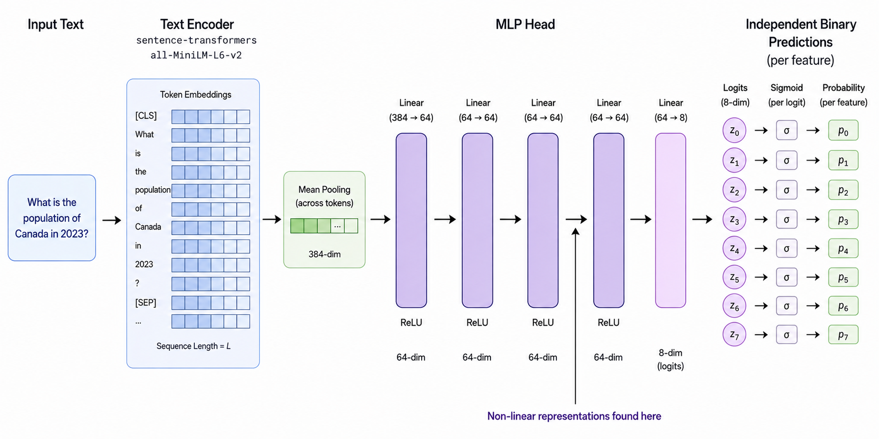
Figure 1: Architecture diagram of the model given for the BlueDot Safety Puzzle. Arrow highlights the activations of the classifier to be investigated.

The problem was structured into 3 parts:

• Task 1: Identify which class was not linearly separable at the given point in the network.
• Task 2: Identify the geometric representation in activation space of this non-linear feature.
• Task 3: Train a similar network with a “more interesting” geometric representation (where “more interesting” is in the eye of the beholder).

On 14th June we had confirmation that our solution to the first two tasks was correct. If you’d like to hear more about how we tackled those, please reach out (spoiler: it’s classic mechanistic interpretability - poking around in activation space and looking for patterns - something that we’re big fans of here!)

For now though, this blog post focusses on the “stretch goal” of training interesting representations into the activation space (Task 3).

Minimising the CamuLoss

Over the course of the work in Task 1 and Task 2, the question we kept in mind was “How did the problem setters actually achieve this?”. A few possibilities came to mind, but the one that seemed most feasible (and extensible) was that an auxiliary term was added to the loss function at train-time which forced this interesting behaviour. Under this assumption, we had an idea for a way that we could use the same technique in order to do something interesting.

We construct the following loss function:

$L = L_C + \lambda_{geom} L_{geom} + \lambda_{res} L_{res} + \lambda_{var} L_{var}$

Where $L_{C}$ is the standard BCE classification loss, $L_{geom}$ is a multi-scale Maximum Mean Discrepancy [2] loss term that operates on the layer 3 activations, $L_{res}$ is the sum of squared residuals from a defined plane in the layer 3 activations, $L_{var}$ is a variance ratio term (between on-plane and off-plane variance) that encourages the defined plane to explain most of the variance and $\lambda_{geom}$, $\lambda_{res}$, $\lambda_{var}$ are tunable weightings for the geometric, residual and variance terms respectively.

The combination of $L_{res}$ and $L_{var}$ constrains the layer 3 activations to primarily lie on a 2D plane in activation space (though in practice, we use small values for $\lambda_{res}$ and $\lambda_{var}$ (0.001 and 0.1, respectively)), and increases the chance of a 2D PCA discovering this plane. The more significant term in this loss function is $L_{geom}$ (with a $\lambda_{geom}$ of 30). This term constrains the activations within the 2D plane, such that they conform to a given distribution. For what follows, we have chosen to add our “interesting representation” to the country feature. At train time, country=1 activations are matched to one distribution, whilst country=0 activations are matched to a different one. This encourages positive activations to occupy one region on the plane, whilst negative activations occupy a different region. The “multi-scale” aspect of the $L_{geom}$ loss term computes the average MMD loss over a range of different kernel bandwidths. Small bandwidths preserve fine distribution details, whilst large bandwidths align the broad distribution, encouraging the 2D representation of the activations to conform to both coarse- and fine-grained detail in the target distribution. Importantly, the MMD loss does not pair each sample with a given point on the plane, but rather matches just the distributions on the plane. This means the classifier can retain some flexibility whilst being encouraged to encode country geometrically as membership in a specific 2D region.

The custom loss function looks as follows (this is pseudocode, reach out if you want to see the full thing):

class CamuLoss(nn.Module):
	def __init__(
		self,
		hidden_dim,
		target_scale=7.0,
		mmd_weight=30.0,
	):
		super().__init__()
		self.centre = nn.Parameter(torch.zeros(hidden_dim))
		self.target_scale = target_scale
		self.learnable_basis = learnable_basis
		self.mmd_weight = mmd_weight

	def orthonormal_basis(self):
		if self.learnable_basis:
			return torch.linalg.qr(self.raw_basis).Q
		return self.raw_basis

	def _multiscale_mmd(self, z_pred, z_target):
		squared_pred = torch.cdist(z_pred, z_pred).square()
		squared_target = torch.cdist(z_target, z_target).square()
		squared_cross = torch.cdist(z_pred, z_target).square()
		bandwidths = z_pred.new_tensor([0.07, 0.15, 0.3, 0.6, 1.2, 2.4])
		losses = []
		for bandwidth in bandwidths:
			denominator = 2 * bandwidth.square()
			losses.append(
				torch.exp(-squared_pred / denominator).mean()
				+ torch.exp(-squared_target / denominator).mean()
				- 2 * torch.exp(-squared_cross / denominator).mean()
			)
		return torch.stack(losses).mean()

	def forward(self, h, z_target, country_labels):
		basis = self.orthonormal_basis()
		h0 = h - self.centre
		z_pred = h0 @ basis
		h_subspace = z_pred @ basis.T
		h_residual = h0 - h_subspace
		class_mmd_losses = [
			self._multiscale_mmd(z_pred[mask], z_target[mask] * self.target_scale)
			for country_value in (False, True)
			if (mask := country_labels.bool() == country_value).any()
		]
		mmd_loss = torch.stack(class_mmd_losses).mean()
		coord_loss = self.mmd_weight * mmd_loss
		residual_loss = h_residual.square().sum(dim=-1).mean()
		residual_variance = h_residual.var(dim=0, unbiased=False).sum()
		subspace_variance = h_subspace.var(dim=0, unbiased=False).sum()
		variance_ratio_loss = residual_variance / (subspace_variance + 1e-8)
		return coord_loss, residual_loss, variance_ratio_loss

We train our classifier for 500 epochs, and get the following per-class test accuracies:

Class	Accuracy
number	0.97
question	0.99
color	0.96
food	0.97
sentiment	0.97
country	0.99
person	0.99
body_part	0.97

So the final question: what were our target distributions for the country=1 and country=0 cases? We wrote a small helper which, given a black and white PNG, will convert it to a bitmap where white pixels form the positive distribution, and black pixels form the negative distribution:

def load_bitmap_targets(image_path, threshold=128, foreground="light"):
    def _normalise_pixel_coordinates(mask):
        rows, cols = np.nonzero(mask)
        height, width = mask.shape
        x = cols.astype(np.float32)
        y = (height - 1 - rows).astype(np.float32)
        if width > 1:
            x = 2.0 * x / (width - 1) - 1.0
        else:
            x = np.zeros_like(x)
        if height > 1:
            y = 2.0 * y / (height - 1) - 1.0
        else:
            y = np.zeros_like(y)
        return torch.tensor(np.column_stack([x, y]), dtype=torch.float32)

    img = Image.open(image_path).convert("L")
    bilevel = img.point(lambda pixel: 255 if pixel >= threshold else 0, mode="1")

    grayscale = np.asarray(bilevel.convert("L"))
    foreground_mask = grayscale < threshold if foreground == "dark" else grayscale >= threshold
    background_mask = ~foreground_mask
    foreground_coords = _normalise_pixel_coordinates(foreground_mask)
    background_coords = _normalise_pixel_coordinates(background_mask)
    return foreground_coords, background_coords

Figures 2 and 3 show views of the 2D PCA of the layer 3 activations with country=1 shown in green, and country=0 in grey:

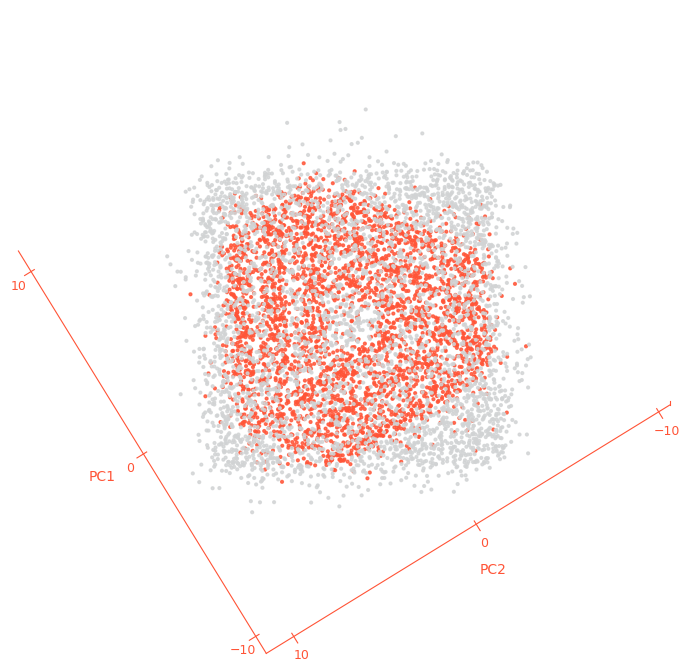
Figure 2: PCA projection of layer 3 activations of our classifier, country=1 shown in green, country=0 shown in grey. country=1 points lie on a distribution that matches the Camulos logo.

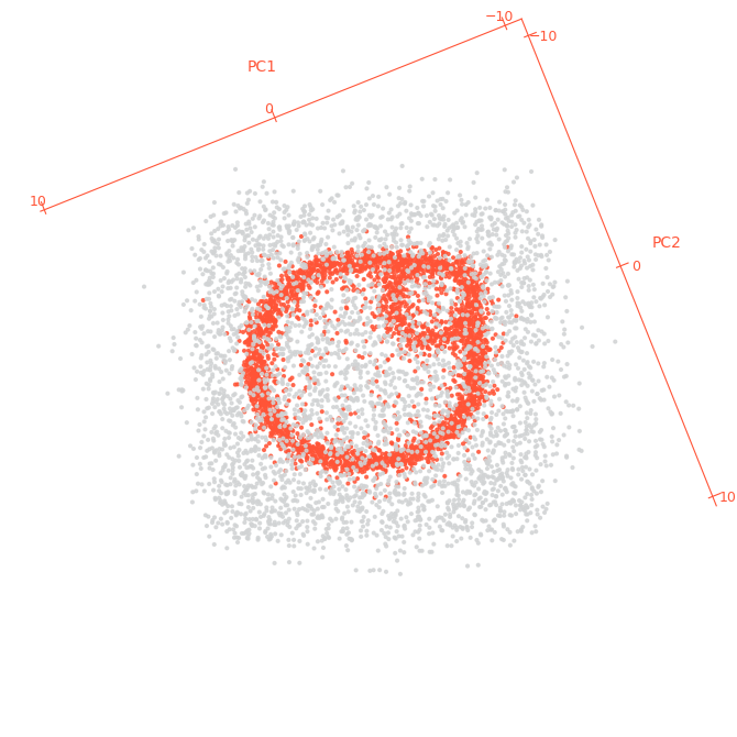
Figure 3: PCA projection of layer 3 activations of our classifier, country=1 shown in green, country=0 shown in grey. country=1 points lie on a distribution that matches the BlueDot Impact logo.

Conclusion

It was a fun little project, and was interesting getting to work on a contrived problem where you know something is amiss, but just need to find out what exactly. Our thanks to the BlueDot team for putting something so fun together! Getting the logos embedded in the activations was also a particularly fun challenge, even if slightly silly.

Having said that, we think there could be some interesting work in using similar techniques to watermark the internal behaviours of models, rather than the outputs. For example: being able to detect that a model has been distilled by a competitor by showing that the competitors model matches an activation distribution that you intentionally trained into your model1, following from the work of Blank et al. that found sublimial learning was mediated by distillation of a single steering vector [3].

If you’re interested in any of this work, or would like to chat more about mechanistic interpretability, please do reach out!

1. or even understanding if such a thing is possible. ↩

References

1. BlueDot. “Technical AI Safety Puzzle #1.” https://bluedot.org/puzzles/technical-ai-safety
2. Gretton, Arthur, et al. “A kernel two-sample test.” The Journal of Machine Learning Research 13.1 (2012): 723-773.
3. Blank, Camila, et al. “Subliminal Learning Is Steering Vector Distillation” https://arxiv.org/abs/2606.00995